Calibration Curve Calculator

Calibration Curve Calculator for unknown samples

A calibration curve connects known standard concentrations to measured instrument signals. The calculator uses your standard table to fit a straight line. It then uses that line to estimate the concentration of an unknown sample.

This tool works best when the assay response is linear across the standards you entered. A typical spectrophotometer, plate reader, or colorimetric assay can use this workflow when the signal increases in proportion to concentration. The signal can be absorbance, fluorescence, luminescence, peak area, or another numeric response.

Students can use the calculator to check homework on standard curves and linear regression. Teachers can use it to show how a calibration line converts signal into concentration. Lab workers can use it for quick educational checks before reporting assay values. Researchers can use it to screen whether standards and unknowns sit inside the useful linear range.

The calculator does not replace a validated assay method. It assumes that the standards and the unknown were measured under the same conditions. It also assumes that a straight-line model is appropriate for the selected range.

Calibration Curve Calculator formula

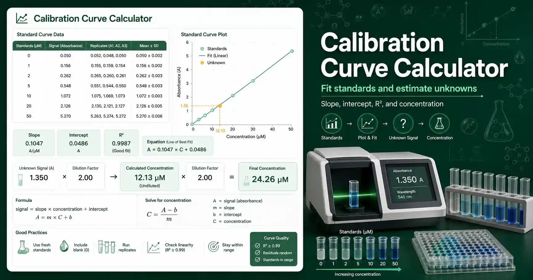
The fitted line has the form signal = slope × concentration + intercept. The slope tells you how much the signal changes per unit concentration. The intercept estimates the signal when concentration is zero.

To calculate the unknown concentration, the calculator rearranges the line to concentration = (unknown signal − intercept) / slope. If you enter a blank signal, the calculator subtracts it from every standard and unknown reading before fitting the line. If you enter a dilution factor, it multiplies the calculated concentration by that factor.

Use the Beer-Lambert Law Calculator when you know molar absorptivity and path length. Use this calibration curve tool when you have measured standards and want the instrument response to define the relationship. The two approaches are related, but a standard curve often handles real assay behavior more directly.

For a broad explanation of calibration curves in analytical chemistry, Chemistry LibreTexts provides a useful educational overview of linear regression and calibration curves. Always match any online explanation to the specific assay, instrument, and validation rules used in your class or lab.

Calibration Curve Calculator result interpretation

The slope, intercept, and R² should be reviewed together. A positive slope usually means the signal rises as concentration increases. A small intercept can be acceptable when the blank and baseline are well controlled. A large intercept may suggest blank error, background signal, reagent carryover, or a nonzero baseline.

R² measures how closely the standards follow the fitted line. A value near 1.000 supports a strong linear fit. It does not prove that the assay is accurate, and it does not prove that extrapolated unknowns are reliable. A sample outside the standard range should be diluted, concentrated, or re-measured with a wider set of standards when possible.

Rounding matters because standard curve results can look more precise than the assay really is. Report enough digits for useful lab work, but avoid implying more accuracy than the standards support. If standards were prepared to two or three significant figures, the final concentration should usually follow similar precision.

Blank correction matters when the solvent, reagent, plate, or cuvette has background signal. A blank value that is too high can create negative corrected signals. A blank value that is too low can inflate every calculated concentration. Check the blank before trusting the final unknown result.

Calibration Curve Calculator for absorbance assays

Absorbance assays often use calibration curves when the molar absorptivity is unknown or when the assay chemistry changes the measured signal. A protein assay, dye assay, ELISA plate, or colorimetric reaction may not follow a simple theoretical equation across every concentration. A measured standard curve helps connect the actual instrument signal to known values.

For ELISA work, a linear curve may be useful over a narrow range, but many ELISA datasets use nonlinear models. The ELISA Standard Curve Calculator is a better related tool when the response is sigmoidal and needs a dedicated standard curve workflow. Choose the model that matches the biology, chemistry, and assay instructions.

Common mistakes include mixing units between standards, entering diluted standards as final concentrations, forgetting to apply a dilution factor to the unknown, and using an unknown signal above the highest standard. Another common mistake is keeping a saturated point in the standard curve. Saturated readings can bend the curve and distort the slope.

Verify critical lab calculations independently before using them in real experiments. Check standard preparation, pipetting records, blank handling, instrument settings, and assay linear range. A calculator can reduce arithmetic errors, but it cannot detect every experimental mistake.

Calibration Curve Calculator worked example